Final Assignment

Donahue and Levitt present a relatively convincing argument for a link between abortion and crime rate. However, before I go into detail about their article, it is pertinent that I discuss how Freakonomics treats the work. Obviously, with one of the authors of the article also being an author of Freakonomics, the chapter pays a close attention to the article as written by Donahue and Levitt and little about the criticisms from the comment by Foote and Goetz. That is far from saying that the chapter in the book devoted to this topic is not with merit.

Dubner's style of writing is able to put a particular spin on something that would be of a boring nature to the average reader. He is able to make the topic of the link between abortion and crime rate an accessible one. To begin the chapter with an anecdote to the story of Romania makes for understanding the reverse of what happened in America in the past few decades; ie criminalized abortion and high crime rate. The chapter treats the topic of Donahue and Levitt's paper in full following this anecdote by providing reasons for why other suggestions of why the crime rate has dropped so significantly in the 90's just doesn't pan out. It then of course poses a decent summary in well versed prose of Donahue and Levitt's findings.

Donahue and Levitt's article of course posits that there is a relationship between abortion and crime rate, potentially a causal one, and that the legalization of abortion in the early 70's can explain at most 50% of the drop in the crime rate in the 90's. If true, this is indeed a significant find. Donahue and Levitt achieve this by analyzing differences in states that legalized abortion before Roe v. Wade, against states with abortion illegal. Likewise, they compare trends before the historic 1973 Supreme Court case and after, finding that the cohort born after the legalization of abortion was less likely to contribute to violent crime compared to the pre-legalization cohort. Comparisons within states also seemed to reveal a negative relationship between abortion and violent crime rate. The most interesting part of this study is actually how it analyzes the different cohorts, and is able to find that the cohort affected by Roe v. Wade had less crime on average than the cohort born before it.

Foote and Goetz's comments are of course concerning. The most startling realization I had from reading their comments was to consider the effect the cross sectional data would have on Donahue and Levitt's results. It doesn't entirely make sense to compare cohorts across states, many of which have several different demographic make ups and of course different laws which might affect crime rates outside of the model that was considered in Donahue and Levitt. The comment that the in-state regression is flawed from a coding error, which after being corrected Foote and Goetz found no relationship between abortion and crime, is also concerning as it raises the issue of the validity of Donahue and Levitt's results.

It is difficult to reconcile Foote and Goetz's comments with the chapter four of Freakonomics. The book never truly analyzes the problems with cross sectional data, nor does it address the concern posited by Foote and Goetz that there is a coding error in the regressions presented in Donahue and Levitt. That said, the comments by Foote and Goetz do not make Donahue and Levitt's model entirely invalid. Foote and Goetz were unable to prove false the cross sectional regressions done by Donahue and Levitt, other than positing that the effect might by due to the nature of the cross sectional data rather than any actual link between abortion and crime. However, they were unable to show this. Therefore, Donahue and Levitt's model does indeed have some validity, as Foote and Goetz cannot fully reconcile the weakness of cross sectional data and the results in Donahue and Levitt, nor do the posit other possible explanations for the reason as to why crime rates have dropped so significantly in the past few decades.

Assignment 10

This chapter presents a series of arguments surrounding the concept of microcredit. Statistically speaking, and in comparison with the other chapters, this one seemed to be a bit of a wash. The first statistic that the reader is presented with is one that highlights the difficulties the poor face when it comes to lending.. The statistic itself deals with the interest rate in real terms as evidence that the poor on average overpay for loans. The best thing the authors do recently in the book (which happens with this statistic, which is why I am mentioning it only and not the several others presented throughout the chapter) is how the authors bring the reader back to understand what the statistic is saying and the meaning of the statistic. In terms of the interest rate statistic, the author's provide us a little idea of what it would be like to be poor and borrowing from (potentially shady) alternative sources of credit. Using American dollars (and therefore values that the reader can compare, it can quickly be seen how fast the interest on these loans blows up and become un-affordable.
As usual with these authors, statistics is presented i a certain way. First, a topic is semi-introduced (even if it is only a minor issue in the chapter) an engrossing statistic is used either to upset the reader or will be referenced again because the statistic is wrong.

Assignment #9

Neal (1995) examines the wage-cost of switching industries among displaced workers. Neal finds evidence that suggests the wage-cost of workers switching industries is highly correlated with both work experience and tenure in their previous job. Workers who switch industries and have high industry-specific capital are faced with lower wages in general in their newer job, and for workers who remain in their predisplacement industry, firm-specific human capital does not play as large a role in wage determination as does industry-specific human capital.

The largest implication of this paper on my research so far is that industry might play a large role in determination of how long one might stay in the job search following termination. Industries that in general have more competitive job markets might influence individuals to stay in the job search longer than their counterparts, as they would not risk switching to another industry and incurring lost wages. Another insight is that a focus on firm-specific human capital might be too narrow, and industry-specific human capital should be included as well.

With regards to problems of the classic OLS regression, the largest problem might be the cross sectional data that I have (heteroskedasticity), and the possibility of selection bias. To get around this problem, Neal uses a variant of Heckman's (1979) two stage procedure to produce the corrected versions of his regressions and thus control for selection bias. Neal continues by estimating selection equations and is able to effectively control for any possible selection bias. It is possible that I could correct for the cross sectional issue by using a time-series variant of my data, but it'll require some looking in to.

References

Neal,Derek. "Industry-Specific Human Capital: Evidence from DisplacedWorkers." Journal of Labor Economics 13.4 (1995): 653-77. Print.
 

Preliminary Regression Results

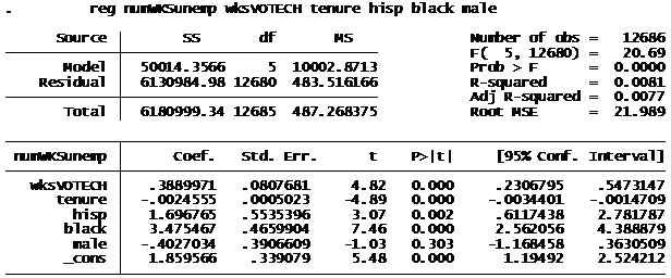
This is currently my best regression result that I have obtained so far. For those not familiar with what I'm currently working on, I'm interested in seeing what the relation is between firm specific human capital and employment outcomes following job termination. Basically, I would expect for those individuals with large amounts of job training to experience more time in unemployment following termination.

wksVOTECH is a proxy for firm specialization, and is the number of weeks spent in any training or vocational programs for the employee's job. Tenure is the number of weeks spent at the job, hisp is a dummy for Hispanic race, black is a dummy for black, and male is a dummy controlling for gender. numWKSunemp is the total number of weeks spent in unemployment following termination from a primary job, and is being treated as the response variable in this model.

At first glance it would appear that wksVOTECH is positively correlated with numWKSunemp. However, two problems exist. First, the r-squared is exceptionally low, below 0.01. Thus, this model is not a good fit of the data at all. Why is this the case? Unfortunately, it's the sample size. It's the entire NLSY79 cohort, which is the data set that I'm working from. Therefore, there are several non-responses, and response errors in general that are affecting my results. Several data points are thus unnecessary. My attempts at filtering them out simply did not work. In short, these results are meaningless.

Going forward, I would like to (correctly) filter out the unnecessary data that is unintentionally affecting my results, attempt to create new variables that are summations of others (not summation as in addition, but placing one variable and another together to create one variable with a larger number of observations). After this, I believe I can include my remaining variables that I have not yet included; an industry breakdown and educational attainment. 

Assignment #7

In chapter 4 of Poor Economics, the authors evaluate the idea of an education poverty trap. The authors go on to show how education varies wildly across the developing world. For example, poor nations in Africa attempt to improve education by increasing the availability of schooling, yet this does not seem to improve education. This is used as a lead-in to highlight two opposing views on the education debate: supply-side and demand-side. Supply-siders would state that the issue lies on the supply of education, so governments need to provide better quality education in the form of better teachers, schools, and the availability of all these education resources. Demand-siders differ in that parents would demand better education if there was an actual incentive for better education (i.e. higher-paying jobs).

In a recent blog in the Huffington Post, Is Education the Way Out of the Poverty Trap?, Dan Haesler takes the supply-side view while discussing the education state of poverty-stricken children in Australia. The post makes use of statistics mainly as lead-ins to discuss its ideology of how to fix the problem. For example, the first meaningful statistic is used to show the level of child-poverty in Australia, at about 12% (which is 12% of Australian children who live in a house where the family income is half the median wage). It then goes on to cite external research that shows how socioeconomically deprived boys disengage from the public education system at about 7 or 8 years of age. What the article does not do, which I would like to see more of, is to attempt to give meaningful statistics related to possible implementations of what the author suggests to be remedies for the country's education problem. Specifically, the article mentions that better teachers are needed on whole who can actively engage students to make them interested and see the need in learning. The article's choice criticism of one of Australia's programs at helping educate deprived areas and the program Teach for America, falls short of being meaningful as the support for the author's criticism lies with his conjecture that most of the teachers in the program quit the program after two years.

Unfortunately the comments on this linked article are closed.

Introduction (Tentative)

Introduction (highly tentative)

Since Becker first posited the theory of human capital, there have been many vaugeries as to what might be the results of his wide reaching theory. Here, I examine the effects of firm-specific human capital on job turnover. Firm-specific human capital is capital that a worker acquires from training by or at the firm to achieve tasks entirely related to one's own firm. In this case, human capital would predict that such capital attainment is risky. This is because at high levels of firm-specific human capital attainment, a worker becomes so specialized that it is hard to transfer their skills to another job. In this case, I expect that workers with large amounts of human capital should face longer job search length during unemployment following dismissal or quitting their previous job.  

Something strange happened when I pasted my bibliography (which also is continuously growing as I find more research related to my topic) to cause the line spacing to be inconsistent. Please forgive me. 

Bibliography

Edward P. Lazear. "Firm‐Specific Human Capital: A Skill‐Weights Approach." Journal of Political Economy 117.5 (2009): 914-40. Print.

Felli, Leonardo, and Christopher Harris. "Learning, Wage Dynamics, and Firm-Specific Human Capital." Journal of Political Economy 104.4 (1996): 838-68. Print.

Jovanovic, Boyan. "Firm-Specific Capital and Turnover." Journal of Political Economy 87.6 (1979): 1246-60. Print.

Neal, Derek. "Industry-Specific Human Capital: Evidence from Displaced Workers." Journal of Labor Economics 13.4 (1995): 653-77. Print.

Parsons, Donald O. "Specific Human Capital: An Application to Quit Rates and Layoff Rates." Journal of Political Economy 80.6 (1972): 1120-43. Print.

Assignment #5

The main thesis of this chapter in Freakonomics is that the notion of the average high-earning drug dealer is wrong. In reality, it is only a small portion of those in the illicit business that are high earners, while the rest barely make a living. Statistics used by Levitt and Dubner to support this argument are presented through the reader slowly throughout the chapter to both build this argument (although it is not first explicitly stated in the chapter, except by reading the title of the chapter) and increase shock value.

First, we see the pyramidal structure of drug organizations:
Pg. 99, 20% of the Black Disciples revenues are sent to the "Board of Directors" for right-of-sale

Next, we see the total monthly revenues of the Black Disciples while Venkatesh was looking at the books:
Pg. 100, Monthly Revenue is $32000

On pg. 102., we see that the gang leader takes a large payout for leading his gang.
Pg. 102, Monthly earnings for J.T.: $8500

By comparison, we see that the majority of drug dealers, foot soldiers, earn very little"
Pg. 103, foot soldiers make $3.30/hour

These statistics achieve several goals. First, the organizational structure of the gang dispels the notion of a grassroots drug dealership, in which the actual drug dealers take home the majority of the profit. Likewise, we see that while the operation is highly profitable, most of the profits don't go to the actual drug dealers, but the leaders. Lastly, we see how very little the actual drug dealer, or foot soldier earns, and it's less than minimum wage.

The presentation of the statistics in this order makes for a very readable and fairly understandable argument that the majority of drug dealers are not wealthy Tony Montana's, but poor below minimum wage earners who might work several jobs besides being a foot soldier to make ends meet. That said, the viability of the statistics is questionable. First, the data is merely from the books of one Chicago-based gang. It is also questionable how much of the books that Venkatesh got his hands on are indeed the legitimate operations of the gang or forgeries That said, these statistics are fairly believable. Why would we ever expect the foot soldier of a gang, who does the actual day-to-day selling of the product, to make the most money in the gang. Furthermore, why would we even expect them to even make decent money? It makes sense to see that the foot soldiers of a gang make next to nothing, while the small top tier takes the largest portion of the profits. In an illicit business such as this, it only makes sense that those who run the organization would receive the largest share of the profits as opposed to the average worker/dealer.

References

Friday, March 22, 2013